Bayes theorem

Thomas Bayes (1702-1761)

In probability theory Thomas Bayes is legendary for his theorem (known as Bayes theorem). which can be written thus:

Pr(x,y) = Pr(x│y) Pr(y) = Pr(y│x) Pr(x)

Pr(x) ≡ ∫dy Pr(x,y)
Pr(y) ≡ ∫dx Pr(x,y)

where Pr(x,y) is the joint probability of a pair of vectors x and y, Pr(x) and Pr(y) are marginal probabilities of the single vectors x or y (respectively), and Pr(x│y) and Pr(y│x) are conditional probabilities defined from the above as

Pr(x│y) ≡ Pr(x,y) / ∫dx Pr(x,y)
Pr(y│x) ≡ Pr(x,y) / ∫dy Pr(x,y)

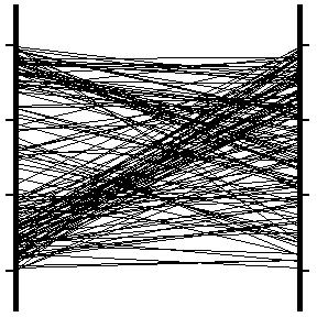
These relationships can be intuitively explained using diagrams. Thus choose state spaces for x and y that each have 3 discrete states, so the total number of joint states is 9. Choose a 3 by 3 matrix of joint probabilities Pr(x,y), and from Pr(x,y) independently draw 150 samples of (x,y) at random.

Now represent each of these samples in the diagram below as a line joining one of the 3 bins on the left (the x-bins) to one of the 3 bins on the right (the y-bins). Vertically jiggle the positions of the end points of the lines so that they don't accidentally fall on top of each other. The number of lines (joining any pair of bins) in this diagram represents the corresponding element of the joint probability Pr(x,y), for each of the 9 (=3*3) possible pairs of bins.

Now display in the diagrams below the contributions that are anchored in each of the 6 (=3+3) possible bins. The number of lines (joining any pair of bins) represents the conditional probability Pr(y│x) (top row) and Pr(x│y) (bottom row). Note that the total number of lines in each diagram represents the corresponding marginal probability, i.e. Pr(x) (top row) and Pr(y) (bottom row).

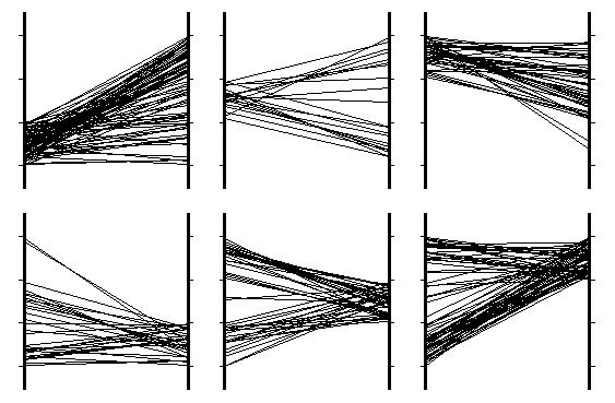
These diagrams give a neat visual summary of the various probability quantities that are interrelated by Bayes theorem. They will provide neat ways of visualising various results that I will describe in future postings to this blog.

Bayesian purists will object to the above diagrams because they rely on drawing a set of samples S from the joint probability P(x,y), and then using S as if it was actually the same object as P(x,y). Of course, they are different objects, but for the purposes of visualisation S is very useful. You can always "fill in the gaps" in your mind's eye.