Vector quantiser simulation

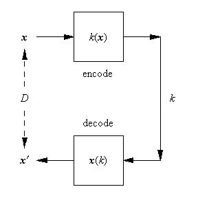
The aim here is to show how to write the code to implement the training of a vector quantiser (VQ) as described in my earlier posting here. The code is implemented as a discrete time dynamical system (DTDS) as described in another of my earlier postings here.

Call in some graphics packages.

Needs["Graphics`Graphics`"];
Needs["Graphics`MultipleListPlot`"];
Needs["DiscreteMath`ComputationalGeometry`"];

Define the size of the training set (i.e. the number of vectors sampled from the input probability density) and the number of code indices to use (i.e. the size of the "code book").

numtrain=100;
numcodes=20;

Define a function nn to compute the index of the vector (in a list of reconstruction vectors r) that lies closest (i.e. is the "nearest neighbour") to an input vector x. This is the encoded version of the input vector.

nn[x_,r_]:=Position[#,Min[#]]&[Map[#.#&[x-#]&,r]][[1,1]];

Read this definition from the inside out:

1. Map[#.#&[x-#]&,r] computes the list of squared distances between the input vector x and each vector in the list of vectors r (the "code book").
2. Position[#,Min[#]]&[...][[1,1]] computes the position in the list of the smallest of the above squared distances.

Define a function y to build a list of the codes corresponding to the whole set of training data at time step t.

y[t_]:=(y[t]=Map[nn[#,r[t]]&,data[t]]);

Read this definition from the inside out:

1. data[t] is a function that returns the training set at time t.
2. Map[nn[#,r[t]]&,data[t]] computes the list of encoded versions of all of the input vectors in the training set.
3. y[t]=... memorises the result of the above step.

Define a function datay to build a list of the training data that maps to each code at time step t.

datay[t_]:=Table[Cases[Transpose[{data[t],y[t]}],{x_,i}:>x],{i,numcodes}];

Read this definition from the inside out:

1. Transpose[{data[t],y[t]}] builds a list of pairs of corresponding input vectors and their codes.
2. Cases[...,{x_,i}:>x] extracts the subset of data vectors that are paired with code i.
3. Table[...,{i,numcodes}] builds a list of the above subsets for all codes.

Define a function r to compute the updated list of reconstruction vectors at time step t.

r[t_]:=(r[t]=Map[If[Length[#]>0,Apply[Plus,#]/Length[#],Table[Random[],{2}]]&,datay[t-1]]);

Read this definition from the inside out:

1. Apply[Plus,#]/Length[#]&[datay[t-1]] computes the updated list of reconstruction vectors from the list of subsets of training data that maps to each code at time step t-1.
2. If[Length[#]>0,...,Table[Random[],{2}]] protects the above code from a possible error codition when the length of a sublist is zero (i.e. none of the training vectors map to a particular code).
3. r[t]=... memorises the result of the above step.

Define the value that the r function returns at time step 0. This initialises the reconstruction vectors.

r[0]=Table[Random[],{numcodes},{2}];

Define a function data that returns the set of training data at time step t. This is a fixed set (for all time steps) of 2-dimensional vectors uniformly distributed in the unit square.

data[t_]=Table[Random[],{numtrain},{2}];

Define the number of training updates. Typically, this VQ converges in far fewer updates than the 20 chosen.

numupdates=20;

Display the training of the reconstruction vectors.

vqgraphics=Table[MultipleListPlot[data[t],r[t],PlotRange->{{0,1},{0,1}},AspectRatio->1,Frame->True,SymbolStyle->{RGBColor[0,0,1],RGBColor[1,0,0]},SymbolShape->{PlotSymbol[Triangle],PlotSymbol[Box]},PlotLabel->"Step "<>ToString[t],FrameTicks->False],{t,0,numupdates}];

[GRAPHICS OMITTED]

Display the encoding cells corresponding to the reconstruction vectors.

codecellgraphics=Table[DiagramPlot[r[t],PlotRange->{{0,1},{0,1}},LabelPoints->False,PlotLabel->"Step "<>ToString[t],Frame->True,FrameTicks->False],{t,0,numupdates}];

[GRAPHICS OMITTED]

Display all of the graphics together.

MapThread[Show[#1,#2]&,{codecellgraphics,vqgraphics}];

[GRAPHICS OMITTED]

Display the first few update steps to show the convergence to an optimum VQ. This example has been chosen deliberately so that it converges fast. It usually takes more than 3 update steps for the optimisation of this VQ to converge.

DisplayTogetherArray[Partition[Take[MapThread[Show[#1,#2]&,{codecellgraphics,vqgraphics}],4],2]];

Because this DTDS implementation of the training of a VQ memorises the values returned by the y and r functions you need to erase these values using y=. and r=. before retraining the VQ.

Basic self-organising network: vector quantiser

The simplest self-organising network (SON) that computes non-linear transformations of data is the vector quantiser (VQ).

A VQ does two simultaneous jobs:

1. Encoding: take each continuous-valued input vector x and use an encoder k(x) to map it to a discrete-valued code k.
2. Decoding: take each discrete-valued code k and use a decoder x(k) to map it to a continuous-valued input x.

Thus a VQ defines a pair of oppositely directed mappings x → k (i.e. k(x)) and k → x (i.e. x(k)). The "quality" of the encoding may be judged by going once round the encode/decode loop thus x → k → x′, and then comparing the original input vector x with its reconstruction x′. A good VQ will have a small reconstruction error, and to achieve this the two mappings k(x) and x(k) must work together harmoniously.

Now let me explicitly show how to optimise a VQ.

A simple measure of the "goodness" of a VQ is a "Euclidean" objective function D that measures the average squared reconstruction error, which is defined as

D = ∫dx Pr(x)║x - x(k(x))║²

where the various pieces have the following interpretation:

1. x(k(x)) encodes (and then decodes) an input vector x to produce a reconstruction.
2. x - x(k(x)) computes the difference between the original input vector and its reconstruction.
3. ║x - x(k(x))║² computes the squared length of the above difference vector.
4. ∫dx Pr(x)║...║² averages the average of the above squared length over input vectors x with probability density Pr(x).

Minimisation of this objective function with respect to the two mappings k(x) and x(k) optimises the VQ.

By inspection, the optimum k(x) is given by

k(x) = argmin_k║x - x(k)║²

Differentiate D with respect to x(k)

∂D/∂x(k) = -2∫dx Pr(x) δ_k,k(x)(x - x(k))

where δ_k,k(x) is a Kronecker delta. The optimum x(k) satisfies ∂D/∂x(k) = 0 (strictly, this is a necessary but not sufficient condition to locate the global optimum) which is given by

x(k) = (∫dx Pr(x) δ_k,k(x) x) / (∫dx Pr(x) δ_k,k(x))

This pair of coupled non-linear equations for the optimum mappings k(x) and x(k) can be solved iteratively.

1. Randomly initialise the x(k) for k = 1, 2, ..., m where m is the size of the "code book" of x(k) vectors to be optimised.
2. Compute the right hand side of the x(k) = (...) / (...) equation, using the k(x) = ... equation to compute k(x) whenever it is needed. The integrals ∫dx Pr(x) (...) are approximated using a finite-sized set of input vectors x (normally called the "training set").
3. The result for (...) / (...) from step 2 above will in general not be the same as the previously assigned values for the x(k). The resolution of this is to overwrite the previous values of the x(k) with the newly computed (...) / (...) from step 2 above, and to iterate this process.
4. When the x(k) have settled down so that successive iterations give (approximately) the same result the optimisation has converged to a minimum of the objective function. Note that this is guaranteed to be a local minimum, but not guaranteed to be a global minimum.

Why is a VQ a SON?

The encoder and decoder pair of mappings k(x) and x(k) bidirectionally connect two spaces (x-space and k-space) thus x ↔ k. The encode/decode loop x → k → x′ contains all the places that k appears, i.e. mapping k(x), k-space, and mapping x(k). The structure of this encode/decode loop is determined entirely by the minimisation of an objective function, and the term "self-organisation" is used to describe the optimisation process that creates the loop x → k → x′. As a side effect of the creation of this encode/decode loop a new space (i.e. k-space) is created that is able to "represent" states in x-space.

This creation of mappings to and from new "representation" spaces is a defining feature of SONs, and the VQ is the simplest example using non-linear mappings that I know of. If the discrete-valued k is replaced by a continuous-valued k, or more generally a vector k, then using a Euclidean objective function the optimum mappings k(x) and x(k) are linear (this is "principal components analysis", or PCA). Note that networks of linear mappings can build only linear mappings, whereas networks of non-linear mappings can build all mappings. It is very convenient that merely using a discrete-valued (rather than a continuous-valued) k or k leads to the useful non-linearity found in a VQ.

This use of discrete-valued quantities turns out to absolutely crucial for building a generalised theory of SONs. I will repeatedly return to this theme in the future.

Quantum mechanics

I have always loved this cartoon which I saw in an old copy of Private Eye. I know it's not about self-organising networks (SON), but QM runs deep in my veins so I thought I would share it.


Actually, SONs and QM are more closely related than you might imagine; I will say more about that in the future.

Discrete time dynamical systems

What is a discrete time dynamical system (DTDS)?

A DTDS is a dynamical system that evolves its state in discrete time steps, rather than through continuous evolution as is usually the case. By choosing a small enough time step a DTDS can approximate a continuous-time dynamical system. All algorithms can be formulated in the language of DTDS, because algorithms are stepwise procedures whose steps can be implemented as individual DTDS time steps. An algorithm running on a piece of hardware is nothing more than a set of rules telling that hardware how to update its state at each tick of the clock. This idea generalises to multiple pieces of hardware with independent clocks.

So DTDS are really useful. How can they be neatly implemented in software?

DTDS are very easy to implement in Mathematica. The archetypal DTDS is a cellular automaton, and where the "universe" consists of an array of discrete-valued cells, and the "laws of physics" consist of a set of cell update rules. A well known example of a cellular automaton is Conway's "Game of Life". More generally, the states of the cells can be anything you want (discrete-valued or continuous-valued), and the update rules can be implemented as any update algorithm you want to apply to the current state of the "universe" of cells. Mathematica has been designed with the simulation of cellular automata in mind, which is why DTDS are very easy to implement in Mathematica.

The Lorenz attractor is a good example to illustrate the implementation of a DTDS in Mathematica.

Initialise a pair of constants. The value of e controls the size of the discrete steps used by the DTDS version of the Lorentz equations to approximate the continuous version of the Lorenz equations.

e=0.013;
r=28;

Define the initial conditions.

x[0]={0.1,0.1,10.0};

Define the Lorenz equations.

x[t_]:=x[t]=
{
  x[t-1][[1]]+10e(x[t-1][[2]]-x[t-1][[1]]),
  x[t-1][[2]]+e(r x[t-1][[1]]-x[t-1][[1]]x[t-1][[3]]-x[t-1][[2]]),
  x[t-1][[3]]+e(x[t-1][[1]]x[t-1][[2]]-(8x[t-1][[3]])/3)
};

The x[t_]:=x[t]=... construct is Mathematica's way of implementing dynamic programming, where the result of evaluating the right hand side of the Lorenz equations is "memorised" using x[t]=..., and then x[t_]:=... can subsequently be used to retrieve this memorised value. This dynamical programming trick ensures that when going from t-1 to t the DTDS memorises its updated state x[t], so that it never needs to recompute x[t].

Call in a graphics package.

Needs["Graphics`Graphics3D`"];

Plot the Lorenz attractor.

ScatterPlot3D[Table[x[t],{t,0,1000}],PlotJoined->True,AspectRatio->1];



Although {x[1],x[2],...,x[1000]} have not actually been evaluated prior to evaluating ScatterPlot3D[...], their evaluation is then forced by evaluating Table[x[t],{t,0,1000}]. In effect the evolution of the DTDS happens as a side effect of asking for its evolution to be plotted. The memorisation of intermediate results using the x[t_]:=x[t]=... construct then ensures that all of {x[0],x[1],x[2],...,x[1000]} are available for immediate reuse, and do not need to be recomputed.

This memorisation of results means that if you want to restart the computation using different initial conditions x[0], then you have to explicitly erase the previously computed values {x[1],x[2],...,x[1000]} otherwise they will not be recomputed based on the new initial condition. An approach that avoids the need to erase values is to enforce the new initial condition on x[1001], and then to carry the computations forwards from there as {x[1002],x[1003],...}. I prefer this latter method because it avoids doing what is effectively a backwards jump in time.

Tag: Mathematica

Including maths in blog postings

In the not too distant future it should be very easy to include maths on web pages in a way that is understood by all web browsers. It is certainly possible to do this right now, but maths is very definitely a second class citizen as far as web pages are concerned.

The technology that helps us to include maths (and other structured objects) on web pages is XML (eXtensible Mark-up Language) which is like a very fancy version of the HTML that we all know and love. I have been tracking the development of XML with interest for many years.

MathML is one of the mark-up languages that has been defined using XML, and its use in blogs has been frequently discussed by Jacques Distler in his blog here. However, I am not aware of any shrink-wrapped solutions to the problem of blogging with MathML. It seems to always require too much hacking around with "utilities", which is something I could do but am too lazy to bother with.

MathML has two features that I very much like:

1. It explicitly represents the full structure of mathematical expressions. This means that it is not a snapshot of the finished equation, but is an algorithmic description of how to construct the equation, keeping the interrelationship between its various parts intact.
2. The maths is part of the web page itself, and is not a set of embedded images (called in from hundreds of small image files) as has been the case in the past (e.g. LaTeX2HTML, Mathematica's "Save as HTML", etc).

Currently few browsers understand MathML directly (e.g. Internet Explorer needs the free MathPlayer plug-in), and even then they do not necessarily display the maths very well. This technology is still not mature.

I particularly like MathML (and more generally XML) because its design allows it to be easily imported/exported to/from Mathematica. The reason for this ease of communication is that the internal representation used by Mathematica is essentially the same as XML.

Mathematica also offers another less pretty way of including maths on web pages, which also preserves the structure of the maths in the same way that MathML does. Thus you can use Mathematica InputForm to write out maths in a 1-dimensional notation. For instance, Sin[x]==Integrate[Cos[x],x] has the obvious meaning, and it will evaluate to True in Mathematica. This approach generalises to arbitrarily complicated expressions but it can become rather "wordy", so careful indenting to highlight the structure of expressions is a good idea.

The use of MathML has not yet become widely enough acknowledged that all web software knows how to display it. For instance, the blog editing software I am using (see www.blogger.com) doesn't understand MathML (or, at least, I can't find a way of doing it). So I will limit myself to using Mathematica InputForm for now in my blog postings.

Functional versus procedural programming

The "functional programming" style that I describe here is not the purist's version of functional programming, where assignment of results to variables does not occur. I have a freer interpretation of the term "functional programming" which is explained by the physical analogy below.

The relationship between functional and procedural programming is succinctly explained by using a physical analogy. Space-time is 4-dimensional and it contains a copy of the 3 spatial dimensions for each and every possible time instant. At each time instant there will be fields recorded throughout the 3-dimensional space, and the evolution of these fields forwards to the next time instant will be governed by whatever laws apply to those fields.

The two styles of programming may then be described thus:

1. Functional programming is the evolution of the fields so that they progressively fill up successive 3-dimensional slices of the 4-dimensional space-time.
2. Procedural programming is the same as functional programming except that at each time instant the 3-dimensional slice containing the evolved copy of the fields overwites the 3-dimensional slice containing the old copy of the fields.

Thus procedural programming reuses storage whereas functional programming does not. A procedural program operates on the state of the world and updates it in place, whereas functional programming makes a copy which it then updates.

A key advantage of functional programming is that the causal chain of updates is laid out explicitly so that an "audit trail" of what has happened during the updates is recorded, whereas in procedural programming this record is overwritten. This means that when a functional program needs to make use of the state of a particular variable at a particular point in time then that state is guaranteed to be available, whereas in a procedural program there is always the danger that the value has been overwritten.

In Mathematica a concrete example of this is as follows:

negativeQ[x_]:=x<0;
f[0]=0;
g[0]=1;
f[t_?negativeQ]:=0;
g[t_?negativeQ]:=0;
f[t_]:=f[t-1]-g[t-1];
g[t_]:=g[t-1]-f[t-2];

where the state of the world at time t is {f[t],g[t]} which depends on the state at the previous two time instants t-1 and t-2. This dependence on various past states is handled completely automatically in functional programming, whereas in procedural programming the overwriting of past states must be carefully buffered in order to ensure that the state at the previous two time instant is available. Clearly, this is a trivial example, but the principle generalises to cases where functional programming is enormously more convenient than procedural programming.

Excessive memory usage by functional programs can be avoided by adopting two strategies:

1. Do as much computation as possible between each time step, because intermediate results that are not assigned to variables are not permanently recorded. The garbage collector will take care of this temporary memory usage.
2. Explicitly erase variables that are no longer required. In effect this creates blank areas in the "audit trail" where parts of the causal chain of updates are "shredded".

Functional programming is a very natural way of writing out discretised evolution equations (as illustrated above). For instance, cellular automata have a completely natural formulation in the functional programming style. More generally, any discretised version of a differential equation can be written out easily in the functional programming style. The key advantage over procedural programming is that you don't need to worry about buffering the past states of the world because they are always available, at least until you erase them.

Functional programming should come naturally to anyone who has been exposed to the space-time way of thinking in physics, where the physicist surveys the whole 4-dimensional record of the world, and thinks in terms of complete histories (i.e. "audit trails").

Mathematica

On www.wolfram.com/products/mathematica it says Mathematica is "The Way the World Calculates". That is sales blurb so I'll allow them a little exaggeration.

It then goes on to say:

"From simple calculator operations to large-scale programming and interactive-document preparation, Mathematica is the tool of choice at the frontiers of scientific research, in engineering analysis and modeling, in technical education from high school to graduate school, and wherever quantitative methods are used."

That is is bit more restrained, and I imagine it is not too far from the truth.

I have been a long-time user of Mathematica since version 1 was released in 1988, and prior to that circa 1980 (when I was doing my PhD on QCD) I used SMP which was the direct ancestor of Mathematica. I cannot exaggerate how much Mathematica has influenced me. It was immediately clear right from version 1 that here was something really new and potentially useful. I say "potentially" because for many years (and versions) I was tantalised by what Mathematica could do in principle, but I was disappointed by its slow compute speed which was a relic of its roots in symbolic algebra. All of these problems have now gone away, and Mathematica is my main tool for technical computing of all sorts, including computationally challenging problems such as image processing. I can do everything I want within one environment, so my "laboratory notebook" is now a hyperlinked web of notebooks containing elements such as text, graphics, maths, software, etc. Apart from idle jottings and scribbles, I have not kept a paper notebook since around 2000. There are no artificial boundaries between the different types of element in Mathematica notebooks which gives me an enormous efficiency advantage over people who don't use Mathematica.

I no longer think of Mathematica as a computer language. It is actually a notation that extends standard mathematical notation into the world of algorithms. Loosely speaking, equations and algorithms are now the same thing for me, because Mathematica is what "breathes the fire into the equations".

I might sound as if I am evangelising about Mathematica, but I am not. I have heard people complain about its price, but that is false economy. It currently costs around £1,600 for a commercial license, much cheaper for teachers, and extremely cheap for students. Based on its productivity and the amount of time you save it pays for itself very quickly.

However, there is a downside. The learning curve for Mathematica is long, especially for people who have used only procedural programming languages (e.g. Fortran, Basic, C++, Matlab, etc) because you have to make a mental shift to the functional programming style. However, these problems are alleviated by the extremely logical and unified structure of Mathematica.

There is another downside that I do find irritating. You need a full Mathematica installation on any computer on which you want to run software that you have written using Mathematica. This means that it is much more difficult to get non-Mathematica users to pay attention to what you are doing than it would otherwise be. Currently it is not possible for you to wrap your software in a standalone EXE. There are various translators that will convert Mathematica to other languages, but they impose strong constraints on what Mathematica constructs you are allowed to use; I have found them to be useless for serious work.

There is a Mathematica newsgroup at comp.soft-sys.math.mathematica where world experts hang out to solve your every Mathematica problem.

I intend to use Mathematica for any code that I might publish in this blog. I will try to ensure that the code can be read as pseudocode by non-Mathematica users, though I will be programming functionally rather than dysfunctionally.

Tag: Mathematica

My online papers

I have a few papers published in arXiv:

1. arXiv.org/cs.LG/0410036: Self-Organised Factorial Encoding of a Toroidal Manifold
2. arXiv.org/cs.NE/0410020: Adaptive Cluster Expansion (ACE): A Hierarchical Bayesian Network
3. arXiv.org/cs.NE/0408050: Invariant Stochastic Encoders
4. arXiv.org/cs.NE/0408049: Using Stochastic Encoders to Discover Structure in Data
5. arXiv.org/cs.NE/0406017: Using Self-Organising Mappings to Learn the Structure of Data Manifolds

I also have an archive of my Crown Copyright publications at www.luttrell.org.uk/papers.

Most of my papers are relevant in some way to the field of self-organising networks.

Tag: arXiv

Reductionism versus emergentism

The issue of reductionism versus emergentism amounts to whether you model your experimental observations in terms of underlying causes (this is reductionism), or whether you directly model the experimental observations in terms of themselves (this is emergentism). There are "wars" waged between the factions that support one or the other approach, with the reductionists being accused of being "coldly scientific", and the emergentists accused of being "vague and mystical". I think this polarisation of attitudes is silly; it seems that people simply like to be partisan and to spoil for a fight.

A concrete example from physics is the modelling of experimental scattering amplitudes using an underlying quantum field theory (QFT), or modelling them directly using an S-matrix approach. QFT (reductionism) predicts the scattering amplitudes from the behaviour of underlying degrees of freedom, whereas the S-matrix approach (emergentism) models the observations directly by defining inter-relationships between the scattering amplitudes.

Reductionism and emergentism are really the same thing, except that they have a different view about what the fundamental degrees of freedom are. Reductionism explains experimental observations in terms of degrees of freedom that are at a deeper level than the experimental observations, whereas emergentism regards the deepest level as being the level at which the experimental observations are made.

A really good book that gives you an informal feel for the issues surrounding reductionism and emergentism is A Different Universe: Reinventing Physics from the Bottom Down by Robert B Laughlin. This book explains why it may not always be useful to use a reductionist approach. Essentially, the up-side of a reductionist model is that it reduces everything to simpler deeper degrees of freedom, but the down-side is that you have to put in the effort to derive everything from these deeper degrees of freedom. Unfortunately, the amount of effort can be prohibitive, in which case the reductionist model explains the observations "in principle", but "in practice" it is too computationally expensive to be useful.

How is all this relevant to self-organising networks?

There are two general classes of network model called "generative" and "recognition" models:

1. The generative class of models are reductionist, because they explain experimental observations in terms of underlying causes (or hidden variables). Usually a generative model is primed in a fair amount of detail, so it contains quite a lot of prior knowledge.
2. The recognition class of models are emergentist, because they compute whatever they need without reference to underlying causes. Usually a recognition model is primed only loosely, so it contains little prior knowledge.

Reductionist and emergentist network models lie at two extremes of a spectrum of possibilities. However, most networks fall close to one or other of these extremes, because each approach has its own "mind set" that tends to repel the other.

The emphasis in this blog is to start with the emergentist approach to SONs, because this approach introduces less prior knowledge, and so is more "hands off" in its analysis of data. It is possible, although not guaranteed, that self-organisation can then be used to automatically discover the sorts of underlying degrees of freedom that are used in the reductionist approach.

If it all goes to plan then reductionism will emerge from emergentism by a process of self-organisation. This sets the scene for my research programme into self-organising networks.

ACEnetica

This is a new blog for discussing ideas about self-organising networks (SON).

The term "ACEnetica" is derived from the phrase "Adaptive Cluster Expansion network", which is what I call my own offering in the field of self-organising networks.

What is a SON?

1. The "N" stands for "network" by which I actually mean a network of interconnected processing nodes, where the global processing activity is broken down into a number of smaller processing activities.
2. The "SO" stands for "self-organising" by which I mean that both the processing at each node and the interconnections between nodes can be adjusted dynamically.

This general definition of a SON covers a wide range of possibilities. However, the only SON approaches that I consider worth discussing in this blog are those that are "scientific"; the rest of the approaches fall into the category of "natural philosophy" which is definitely not the focus of this blog.

This means that the approach must have the following minimal properties:

1. It must be supported by a consistent theoretical framework.
2. It must have predictive power.
3. It must be open to falsification.

There are two levels at which prediction and falsification are done with processing networks:

1. Relationship with the external physical world. This is conventional "science", where the processing network is judged by its ability to explain experimental observations.
2. Relationship with the world of algorithms. This is unconventional "science", and could be called "a new kind of science" (see http://www.wolframscience.com/), where the processing network is judged by its ability to construct processing algorithms.

Some additional properties that are desirable (but not essential) in a SON approach are:

1. It should scale well with network "size".
2. It should include "standard" approaches as special cases.

An extra property that would be a real bonus if it emerged for free:

It explains some (or even all) of the properties of brain-like processing.

In this blog I will attempt to present SONs within the above context.

Tag: ACEnetica