Where is this all going?

You may well wonder where all of this maths is leading us. You will just have to be patient. I am creating the simplest path possible that short-circuits the route to my latest research work. Before long I will be publishing papers in arXiv, and then subsequently discussing them here. When that happens I hope that things will start to get more exciting.

Stochastic vector quantiser

We can now generalise the basic self-organising network known as the vector quantiser by combining results from several earlier postings:

1. In Basic self-organising network: vector quantiser I described a basic type of self-organising network (SON) called a vector quantiser (VQ), which does two simultaneous jobs: Encoding - which takes each continuous-valued input vector x and use an encoder k(x) to map it to a discrete-valued code k, Decoding - which takes each discrete-valued code k and use a decoder x(k) to map it to a continuous-valued input x. This creation of mappings to and from new "representation" spaces is a defining feature of SONs, and the VQ is the simplest example using non-linear mappings that I know of.
2. In Vector quantiser simulation I included Mathematica code for simulating a VQ, which learnt to partition a 2-dimensional regions into "code cells".
3. In Bayes theorem I introduced Bayes theorem for manipulating joint probabilities. This is the key result that makes it possible to do useful computations with joint probabilities, without being constrained to those special cases that admit analytic solutions.
4. In Markov chain Monte Carlo sampling (MCMC) I illustrated how to use Bayes theorem to draw samples from a joint probability, which generates a Markov chain of samples that visits each joint state with a frequency that is proportional to its joint probablity, with the caveat that the sequence thus generates is correlated because it has a memory of its past history.

What do these results give you when they are folded together? The basic result is item 4 above on MCMC sampling joint probabilities. If several MCMC updates are applied to a joint state (x, k) to create the state sequence (?, ?) → (x, ?) → (x, k) → (x′, k), where the MCMC updates alternate between x and k spaces, then the encoding/decoding process that occurs in a VQ can be mimicked, giving the encode/decode loop x → k → x′ that I described in Basic self-organising network: vector quantiser. More generally, if the MCMC updates alternate randomly, then the same VQ encoding/decoding process occurs, but less efficiently.

This connection between VQ encoding/decoding and MCMC algorithms allows a stochastic generalisation of the VQ to be formulated. This is called a stochastic vector quantiser (SVQ), and its structure is shown in the diagram below.

where Pr(k│x) is the encoder's conditional probability over codes k given the input vector x, and Pr(x´│k) is the corresponding decoder's conditional probability.

Compare this diagram with the following two previous diagrams:

1. The basic VQ that I showed in Basic self-organising network: vector quantiser. The only difference is the notation that is used to describe the "encode" and "decode" blocks of the diagrams.
2. The first few updates of the MCMC simulation that I showed in Markov chain Monte Carlo sampling. Each pair of successive diagrams is potentially a stochastic encoding followed by a decoding, assuming that the MCMC algorithm happens to update the right hand space followed by the left hand space.

A slightly more appropriate version of the MCMC diagram would look like the diagram below, where a larger number of states has been used in each of the two spaces than before, and arrows have been drawn to show which space the MCMC algorithm happens to update at each step. In this case the first two steps behave like an SVQ encode/decode loop, because the arrows form the characteristic out-and-back form shown in the SVQ diagram above.

To encode you compute the encoder's conditional probability Pr(k│x), and to decode you then compute the decoder's conditional probability Pr(x´│k). Overall, this specifies the chain x → k → x´ leading from the original input vector, via the code, and then back to a reconstruction of the input vector. Each of the arrows in this chain is stochastic in an SVQ. This means that for each input vector x there is a whole ensemble of alternative possible codes k, each member of which is weighted by the corresponding conditional probability Pr(k│x), and one such member is randomly selected as the coded version of the input. Similarly, for each code k there is a whole ensemble of alternative possible reconstructions x´, each member of which is weighted by the corresponding conditional probability Pr(x´│k). This procedure is equivalent to two steps of an MCMC algorithm.

The SVQ generalisation of the Euclidean VQ objective function is

D = ∫dx Pr(x) ∑_k Pr(k│x) ∫dx´Pr(x´│k) ║x - x´║²

This may be interpreted thus:

1. The joint probability Pr(x, k, x´) of the chain x → k → x´ can be split up as Pr(x, k, x´) = Pr(x) Pr(k│x) Pr(x´│k).
2. ║x - x´║² is the Euclidean distance between the original input vector and its reconstruction after passing along the chain x → k → x´.
3. The ∫dx Pr(x) ∑_k Pr(k│x) ∫dx´Pr(x´│k) (...) sums and integrates over all of the alternative choices of the chain x → k → x´.

By using Bayes theorem this objective function can be simplified to the following

D = 2 ∫dx Pr(x) ∑_k Pr(k│x) ║x - x´(k)║²

where x´(k) is defined as

x´(k) ≡ (∫dx Pr(x) Pr(k│x) x) / (∫dx Pr(x) Pr(k│x))

Compare these expressions with the results in Basic self-organising network: vector quantiser to see that the SVQ and the VQ are mathematically very similar, except that in an SVQ the encoder is stochastic because it is described by Pr(k│x). The overall factor of 2 in the SVQ objective function is not important; it comes from the symmetrical way that I defined D for an SVQ. The VQ is a special case of an SVQ where Pr(k│x) = δ_k,k(x).

Overall, an SVQ is the same as a VQ, except that there is now some "slack" in the choice of how to encode each input vector. Also, a computational structure that is equivalent to an SVQ is embedded within an MCMC simulation of the joint probability Pr(x, k). It turns out that the MCMC viewpoint is ultimately the most useful for making further generalisations of the VQ and SVQ self-organising networks.

One face, one neuron

This month in Scientific American there is a News Scan article entitled One Face, One Neuron, which describes some interesting results (observed in several experimental subjects) in which there was a strong response by a single neuron to fairly abstract concepts. That is to say, when an experimental subject was shown various different things that were related to the same abstract concept, the same neuron fired in each case. It wasn't clear from the article what the rest of the neurons were doing, but there are rather a lot of them so it isn't possible to measure them all.

This observation is really significant, because it means that the brain is mapping a highly variable input onto an invariant response (at least, as far as one of the neurons is concerned), in which a single neuron fires reliably in response to a whole range of inputs. No doubt the neural dynamics that leads to this invariant mapping involves many neurons recurrently interacting with each other, with the net effect being the observed firing behaviour of the single neuron.

How is it that the neural dynamics in the brain can self-organise so that it creates these invariant mappings? Presumably they are something like fixed points (or limit cycles) of the dynamics. What properties of the external input are preserved at the output end of these mappings? In other words, what is the neural code used by the brain? Are the same properties of the external input preserved by different brains? If they are, presumably the detailed mappings are different in different brains. How much can the external input be varied whilst still being mapped to the same output? Is a few vague clues in the external input enough for the recurrent neural dynamics to home in on the appropriate output?

It would be really useful to have a general theory of such self-organising mappings in recurrent networks, wouldn't it?

Laughlin versus reductionism

In a posting Laughlin vs. reductionism Luboš Motl chooses to shoot down Robert Laughlin's book "A Different Universe: Reinventing Physics from the Bottom Down" for its supposed attack on reductionism. I commented before on Reductionism versus emergentism, where I came out in favour of Laughlin's book, because it strikes me as being a fairly balanced account of the merits and disadvantages of reductionism and emergentism. However, my salary is no longer paid to me for doing fundamental physics, so presumably I have less to lose when Laughlin's book damns reductionism with faint praise.

More generally, it is very useful to think at many levels, all the way from deep underlying theories (i.e. reductionism) up to phenomenological descriptions (i.e. emergentism), because useful science can be done at all of these levels, and usually insight at one level can help progress to be made at another level, although this isn't guaranteed.

As I said in Reductionism versus emergentism, my hope is to use self-organising networks to address the relationship between reductionism and emergentism, and "if it all goes to plan then reductionism will emerge from emergentism by a process of self-organisation".

In information processing I certainly do not want to have to think in terms of individual binary digits the whole time. I want to build software objects that have well-defined behaviour at a much higher level, and to be able to ignore the detailed internal workings of these objects, and to deal instead only with their externally exposed properties. However, at the same time, I want to be able to interrogate those higher level properties to discover their internal dynamics. This is what a self-organising network will allow me to do.

You certainly can't do useful (read "macroscopic") self-organising information processing without bumping straight into emergent properties.

Markov chain Monte Carlo sampling

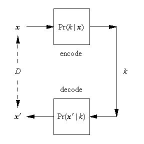
In a previous posting I explained Bayes theorem for splitting up joint probabilities Pr(x,y) into component pieces (either Pr(x│y) Pr(y) or Pr(y│x) Pr(x)), which leads onto a very neat way of drawing sample pairs of vectors (x,y) so that they have the correct joint probability Pr(x,y). This is called Markov chain Monte Carlo (MCMC) sampling.

Firstly, notice that the pair of vectors (x,y) forms a single (higher-dimensional) vector. In the description below this partitioning of the single vector into a pair of vectors (x,y) is done in whatever way is convenient. This will be explained below.

Start off by supposing that someone hands you a pair (x,y) that is known to have joint probability Pr(x,y). You can use this to generate another pair (x,y) that also has joint probability Pr(x,y). Here is how you do it:

1. Use Bayes theorem to split Pr(x,y) as Pr(x,y) = Pr(x│y) Pr(y), where Pr(y) ≡ ∫dx Pr(x,y). This tells you that Pr(x│y) = Pr(x,y) / ∫dx Pr(x,y) which will be used below.
2. Draw a sample vector (call it x´) from the Pr(x│y) computed above, and make this the new value of x. Note that you do not need to know Pr(y) to draw this sample. Here I assume that it is easy to draw an x-sample from Pr(x│y) (e.g. x is low-dimensional) but it is difficult to draw an (x,y)-sample from Pr(x,y) (e.g. (x,y) is high-dimensional) which is the sampling problem that we want to avoid.
3. The joint state is now (x´,y). Its joint probability is Pr(x´│y) Pr(y), where Pr(x´│y) has the same functional dependence on x´ as Pr(x│y) has on x, by construction.
4. Use Bayes theorem to join these together to obtain Pr(x´,y) = Pr(x│y) Pr(y), where Pr(x´,y) has the same functional dependence on x´ as Pr(x,y) has on x, by construction.

The overall effect of the above steps is that (x,y) becomes (x´,y), and the functional form of the joint probability is unchanged by this operation. Excellent! That is exactly what we wanted to do. We now have two pairs of vectors (x,y) becomes (x´,y) sampled from Pr(x,y). The only downside is that the value of y is the same in both pairs of vectors, so they must be strongly correlated with each other.

The partitioning of the whole vector into a pair of smaller vectors (x,y) can be done in any way, and as long as it is easy to draw a sample of x from Pr(x│y) then another (x,y) (different x, same y) can be generated as described above. This process can be iterated (choosing a different partitioning of the whole vector at each iteration) to generate a whole sequence (or Markov chain) of vector samples (hence the name "Markov chain Monte Carlo" sampling) all of which have the correct joint probability. The main caveat is that the sequence is correlated, because each vector in the sequence has a "memory" of the past history of the sequence.

Note that the above algorithm does not work if the initial pair of vectors does not have joint probability Pr(x,y). However, under fairly mild assumptions (i.e. ergodicity), the algorithm will generate a sequence of vectors whose joint probability settles down to Pr(x,y) after an initial convergence period, after which the assumptions of the above algorithm are satisfied.

The diagrams below show how a typical MCMC sequence building up. This uses the same Pr(x,y) and diagrammatic notation as was used in my posting on Bayes theorem here, and was in fact how I generated the diagrams there. A different random seed has been used here. Each of x and y has 3 possible states, so (x,y) has 9 (=3*3) possible joint states.

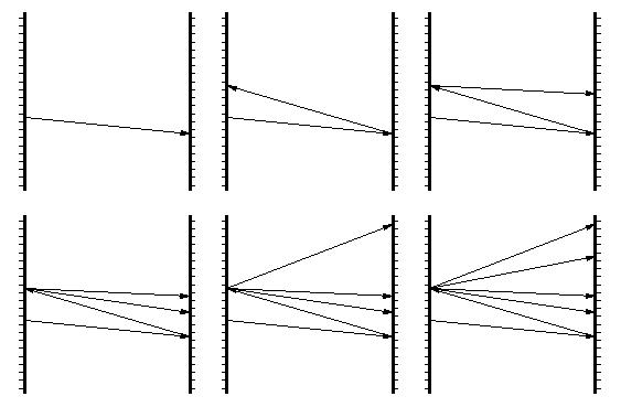
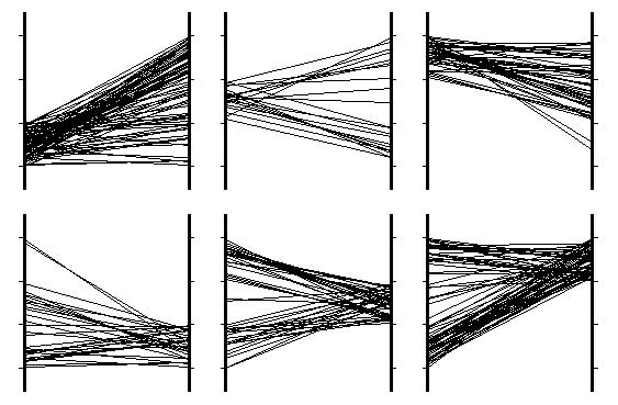
The first diagram shows the first 6 steps of the MCMC sequence, where the initial state (3,2) is at the top left, and successive states are shown in the graphics as read from left to right then top to bottom. After 1 MCMC update the state is unchanged (that is the draw of the random numbers), then after 2 MCMC updates the y part of the state updates so that the state is (3,3), then at the next step the x part of the state updates so that the state is (2,3), then the y part of the state updates so that the state is (2,1), then the next update can't be inferred from the diagram because it repeats a state that occurred earlier. The source of the correlations between successive MCMC samples is clear because each update moves only one end of the line in the graphic.

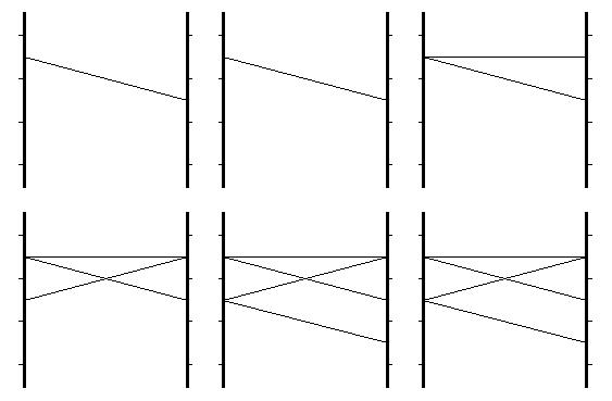
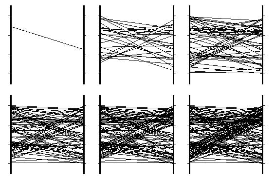
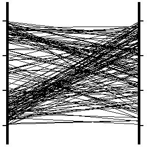
The diagram below shows the same as the diagram above except that 25 MCMC updates elapse between each graphic. Also, for visualisation purposes, the end points of each line representing a joint state are vertically jiggled a little bit so that they don't all fall on top of each other.

This MCMC approach to sampling is very powerful, and with some ingenuity it can be used to draw samples from any joint probability, but always with the caveat that the sequence is correlated.

Bayes theorem

Thomas Bayes (1702-1761)

In probability theory Thomas Bayes is legendary for his theorem (known as Bayes theorem). which can be written thus:

Pr(x,y) = Pr(x│y) Pr(y) = Pr(y│x) Pr(x)

Pr(x) ≡ ∫dy Pr(x,y)
Pr(y) ≡ ∫dx Pr(x,y)

where Pr(x,y) is the joint probability of a pair of vectors x and y, Pr(x) and Pr(y) are marginal probabilities of the single vectors x or y (respectively), and Pr(x│y) and Pr(y│x) are conditional probabilities defined from the above as

Pr(x│y) ≡ Pr(x,y) / ∫dx Pr(x,y)
Pr(y│x) ≡ Pr(x,y) / ∫dy Pr(x,y)

These relationships can be intuitively explained using diagrams. Thus choose state spaces for x and y that each have 3 discrete states, so the total number of joint states is 9. Choose a 3 by 3 matrix of joint probabilities Pr(x,y), and from Pr(x,y) independently draw 150 samples of (x,y) at random.

Now represent each of these samples in the diagram below as a line joining one of the 3 bins on the left (the x-bins) to one of the 3 bins on the right (the y-bins). Vertically jiggle the positions of the end points of the lines so that they don't accidentally fall on top of each other. The number of lines (joining any pair of bins) in this diagram represents the corresponding element of the joint probability Pr(x,y), for each of the 9 (=3*3) possible pairs of bins.

Now display in the diagrams below the contributions that are anchored in each of the 6 (=3+3) possible bins. The number of lines (joining any pair of bins) represents the conditional probability Pr(y│x) (top row) and Pr(x│y) (bottom row). Note that the total number of lines in each diagram represents the corresponding marginal probability, i.e. Pr(x) (top row) and Pr(y) (bottom row).

These diagrams give a neat visual summary of the various probability quantities that are interrelated by Bayes theorem. They will provide neat ways of visualising various results that I will describe in future postings to this blog.

Bayesian purists will object to the above diagrams because they rely on drawing a set of samples S from the joint probability P(x,y), and then using S as if it was actually the same object as P(x,y). Of course, they are different objects, but for the purposes of visualisation S is very useful. You can always "fill in the gaps" in your mind's eye.

Mission to build a simulated brain

In New Scientist a while ago there was an article entitled Mission to build a simulated brain begins which describes "An effort to create the first computer simulation of the entire human brain, right down to the molecular level...". It goes on to say "The hope is that the virtual brain will help shed light on some aspects of human cognition, such as perception, memory and perhaps even consciousness", and so on.

"...simulation of the entire human brain"?!!

1. That's rather a lot of neurons, and a mind-boggling number of connections. And that's not even going down to the molecular level. The state of the art is very limited compared to the goals of this project. I assume that the report is slightly inaccurate.
2. For instance, there are detailed computational models of how neurons function, and how they interact in small assemblies; there is the NEURON software for running these simulations. At a much higher level there are also general architectual models of whole regions of the brain.
3. In a few cases there are models that span several scales all the way from the bottom level to a fairly high level. I am thinking in particular of the visual cortex where we have the luxury of addressing the brain directly via the retina (which is effectively a layer of brain tissue). This has led to a very good (relative to other areas of the brain) neural model of visual processing in the brain.

"...and perhaps even consciousness"?!!

1. When I hear the "C" word I reach for my gun! People routinely use the "C" word to inject an air of mystery and importance into what they are saying. The fact is that it is a non-word that is used by people who haven't seriously reflected on what goes on inside their heads.
2. One book (amongst many) that I have found very insightful on this issue is The Artful Universe Expanded by John Barrow, in which he lucidly explains how evolution ensures that the universe imprints itself on the way that we we think. This means that the thing that we think with is not as free thinking as we would like to believe that it is. Is it at all surprising that we feel as if there is an inner light (call it "consciousness" if you want)?
3. Isn't it obvious that evolution ensures that you (whatever you are, human, fish, ant, or whatever) have a sense of "self" to encourage you to survive and reproduce, or have a sense of "host" to make you sacrifice yourself to save the nest? There will be "degrees" of "self" according to the "amount" of "processing" that is used to "implement" it. Yes, there are inverted commas everywhere because the terminology is not precisely defined.

What sort of brain studies should be given more prominence?

There is a lot of research going on near the bottom level, such as modelling neural chemical processes, modelling the dynamics of membrane potentials, modelling the interaction of small assemblies of neurons, etc. This is all very good reductionist work that potentially will lead to a deeper understanding.

However, I can't see much work going on that studies the theory of low-level brain-like processing, although there is a lot of neural modelling work. What do I mean by that? Brain-like processing is massively parallel, which needs its own special kind of "algorithm" that can be distributed across a large number of small interconnected processors. For really large parallel systems (e.g. brains) you can't go in and individually program every processor, but you can envisage the processors having inbuilt behaviours (i.e. a bootstrap program) that allow them to sort out their collective behaviour (i.e. self-organise) to do something macroscopically useful. We certainly need a lot more work on the theory of this type of massively parallel self-organising system.

There is a vast amount of research into what is called "neural networks", but which is nothing of the sort. As with the "C" word above, the "NN" phrase is used to guild otherwise rather mediocre research to make it seem more sophisticated than it is. A better phrase to describe most of this research is "non-linear adaptive filtering". The small subset of "NN" research that uses discrete firing events, rather than firing rates, is much better qualified to be called "NN".

There is the important distinction between supervised and unsupervised training:

1. Supervised training is usually used to guide an adaptive filter so that it approximates an externally specified output. From the point of view of brain-like processing this is not a very interesting type of adaptation.
2. Unsupervised training is much more interesting because it does not require an output to be externally specified, so the adaptive filter must discover for itself something "interesting" about its input; this is like answering an open-ended question, which is much more challenging than a question with a known answer. From the point of view of brain-like processing this is a very interesting type of adaptation.

Too much time is spent on supervised training by people doing what they think is true "NN" research. They are kidding themselves. How do they expect very large networks to be trained when all the external supervisor can do is to guide the network outputs? Is supervised training really going to help the deep inner workings of the network to learn anything useful? Wouldn't it be much better to distribute throughout the network the ability to discover "interesting" structure? Doesn't this sound rather like what unsupervised training is aiming to do anyway?

In Mission to build a simulated brain begins I want to see more theoretical work, especially on abstract brain-like processing and (more specifically) unsupervised training of neural networks that use discrete firing events, which would then guide the modelling work that they hope to do anyway. To understand what a large network simulation is doing you need a theory that is formulated at an appropriate level. It is not always a good idea to drill down to the bottom level of modelling (see my comments on reductionism versus emergentism).

Whither this blog?

I have had look at the various postings that I have made thus far and notice that, although they are "on topic", they are quite variable in their style. Some verge on seeming to be philosophical (e.g. here) whilst others use a fairly demanding level of maths/software (e.g. here), including several future postings that I currently have in draft form. I even had a comment by private email that their "brain started to explode half way through the VQ article"! I had rather hoped I would get all my comments directly to the blog; there seems to be rather a shortage of them. I seem to be talking to myself!

I operate in any (all, some, or none) of these modes of expression, and my writing and maths tends to show it. It will take a while for me to converge on an optimum approach to posting on this blog, but I suspect it will always mix together different styles. I will try to make the maths as self-evident as possible. After all, I don't think you have really understood a piece of maths until it you can explain it in such an intuitively obvious way that people ask why they are paying you do do something so trivial.

I will post software written in Mathematica to illustrate the points I am making. Maybe some (most?) people don't like my choice of computer language, but I have given my reasons for using Mathematica here. It blurs the distinction between maths and algorithms which I think is a big step forwards. This is one of the main purposes of Stephen Wolfram's New Kind of Science.

I don't think I have yet started to put in enough links to the rest of the world, so I can hardly expect other people to link to me (they haven't yet, as far as I know!). I even tried to set up a trackback from one of my earlier postings here to an arXiv paper of mine here. The trackback was received (it appeared on arXiv's "recent trackbacks" page) , but it never got attached to my paper. I guess the arXiv administrators spiked it because it was a self-comment. That's OK, and it is the appropriate policy for arXiv.

I have had a poke around blogspace and I can't find anyone at all who is posting in the area of self-organising networks (or even self-organizing networks!). There are blogs which have to do with self-organising "social" networks, but that isn't what this blog is about. So how do you start off a blogging community in a new subject area? My own areas of expertise span quantum physics as well as self-organising networks, and I intend to show just how inter-related these two areas are in future postings, so at some point my postings will start to look much more like quantum physics. I hope things will start to interest a lot more people then.

Update: The above arXiv trackback eventually appeared a little over a week after I pinged arXiv. Because this was my first such trackback I must have triggered the manual part of the "semi-automated editorial process that approves trackbacks for display". I pinged arXiv with some more trackbacks, and this time they appeared straight away. So it seems that I have been judged to be "worthy". I will use the privilege wisely.